[선형대수] 행렬의 여러 가지 분해(Matrix decomposition) 정리 (EV, SV, LU, Cholesky, QR) #2

 

 

이번 공부는 수학이 아닌 로봇공학을 공부하는 학생의 관점에서 정리했습니다. 수학적인 의미를 깊게 아는 것도 공학에서 중요하다고 생각하지만 이번에는 의미, 용도, 적용사례 정도에 초점을 두고 공부했습니다.

 

 

*늘 그렇듯 틀린 내용이 있을 수 있습니다.

 

 

 

 

 

 

Lower-Upper decomposition(LU decomposition, LU 분해)

어떤 Square matrix A는 다음과 같이 분해할 수 있다.

 

$A=LU$        $L\text{: Lower-triangular matrix}$,   $U\text{: Upper-triangular matrix}$, 

                             $L=\begin{bmatrix}l_{11} &  & 0 \\\vdots  & \ddots &  \\l_{n1} & \cdots  & l_{nn}\end{bmatrix}$,            $U=\begin{bmatrix}u_{11} & \cdots  & u_{1n} \\& \ddots  & \vdots\\0 && u_{nn}\end{bmatrix}$

 

 

※L, U는 unique 하지 않으며 서로 coupled 되어 있다. 한쪽이 결정되면 반대쪽은 unique 하게 결정된다.

 

※LU 분해가 가능한 행렬의 조건을 확실하게 파악하지 못해서 '어떤'이라고 적었다. 일단 현재 찾은 조건은 "Leading principal minors are non-zero"이다. 좀 더 공부해 보고 이 조건이 맞다면 추후 글을 수정할 것이다.

 

※위 조건에 포함되긴 하지만, 일단 full-rank가 아닌 행렬은 LU decomposition이 불가능하다.

 

 

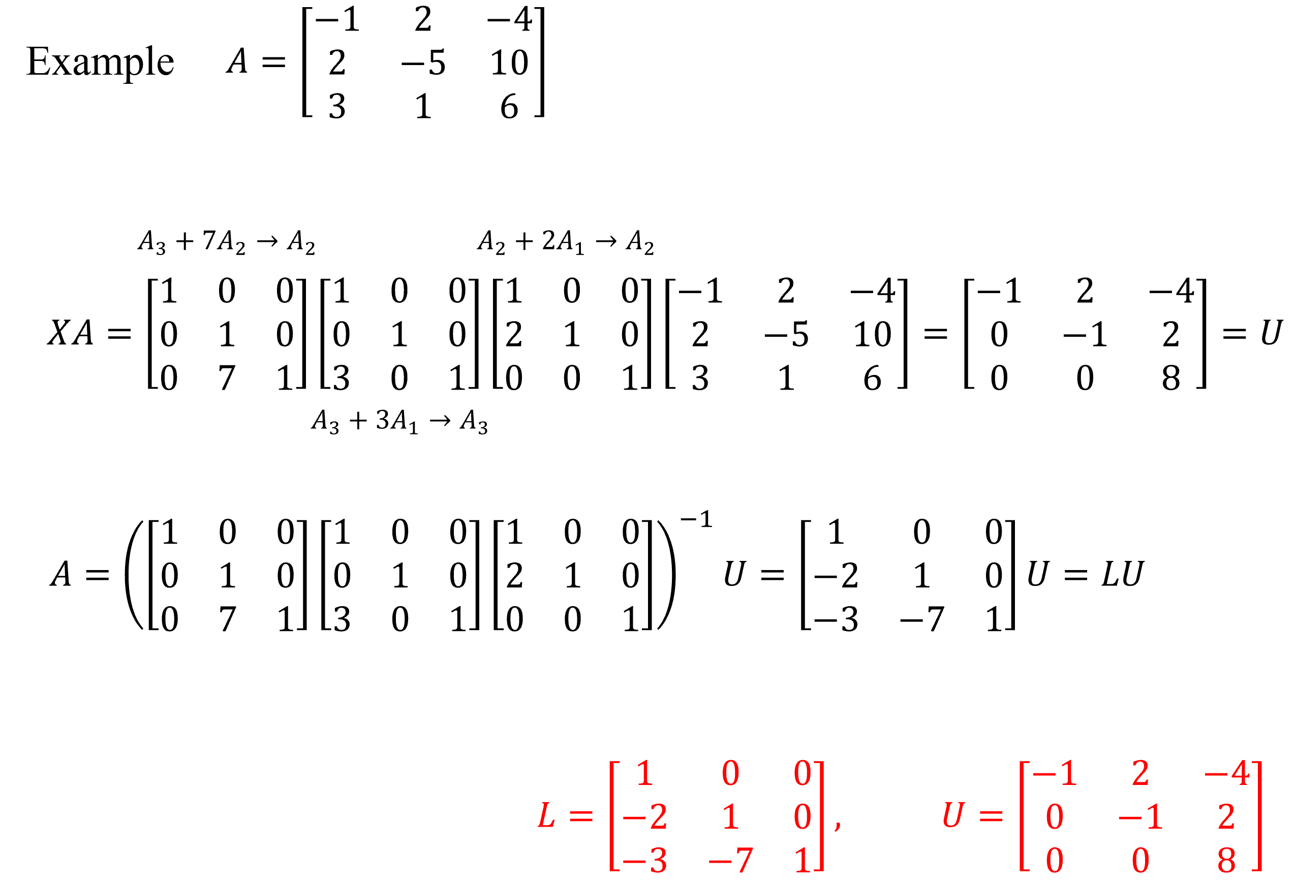
●Pivoting(행 교환)을 사용하지 않는 Gauss elimination(가우스 소거법)과 사실상 같은 과정이다.

 

$A$에 pivoting을 제외한 기본행연산을 해서 upper-triangle matrix $U$로 만드는 과정이 Gauss elimination이며 이는 $XA=U$로 나타낼 수 있다.

 

한편 Gauss elimination 과정에서 기본행 연산의 역행렬 $X^{-1}$은 반드시 lower-triangle matrix가 되므로 $A=X^{-1}U=LU$로 나타낼 수 있고 이 과정이 LU decomposition이다.

 

 

 

※기본행연산과 관련된 것은 "공돌이의 수학정리노트"님의 블로그에 잘 정리되어 있다.

https://angeloyeo.github.io/2021/06/15/elementary_square_matrices.html

기본 행렬 - 공돌이의 수학정리노트 (Angelo's Math Notes)

 

 

 

●모든 Square matrix가 LU decomposition이 가능하지 않지만 pivoting으로 가능하게 만들 수 있다.

 

 

 

 

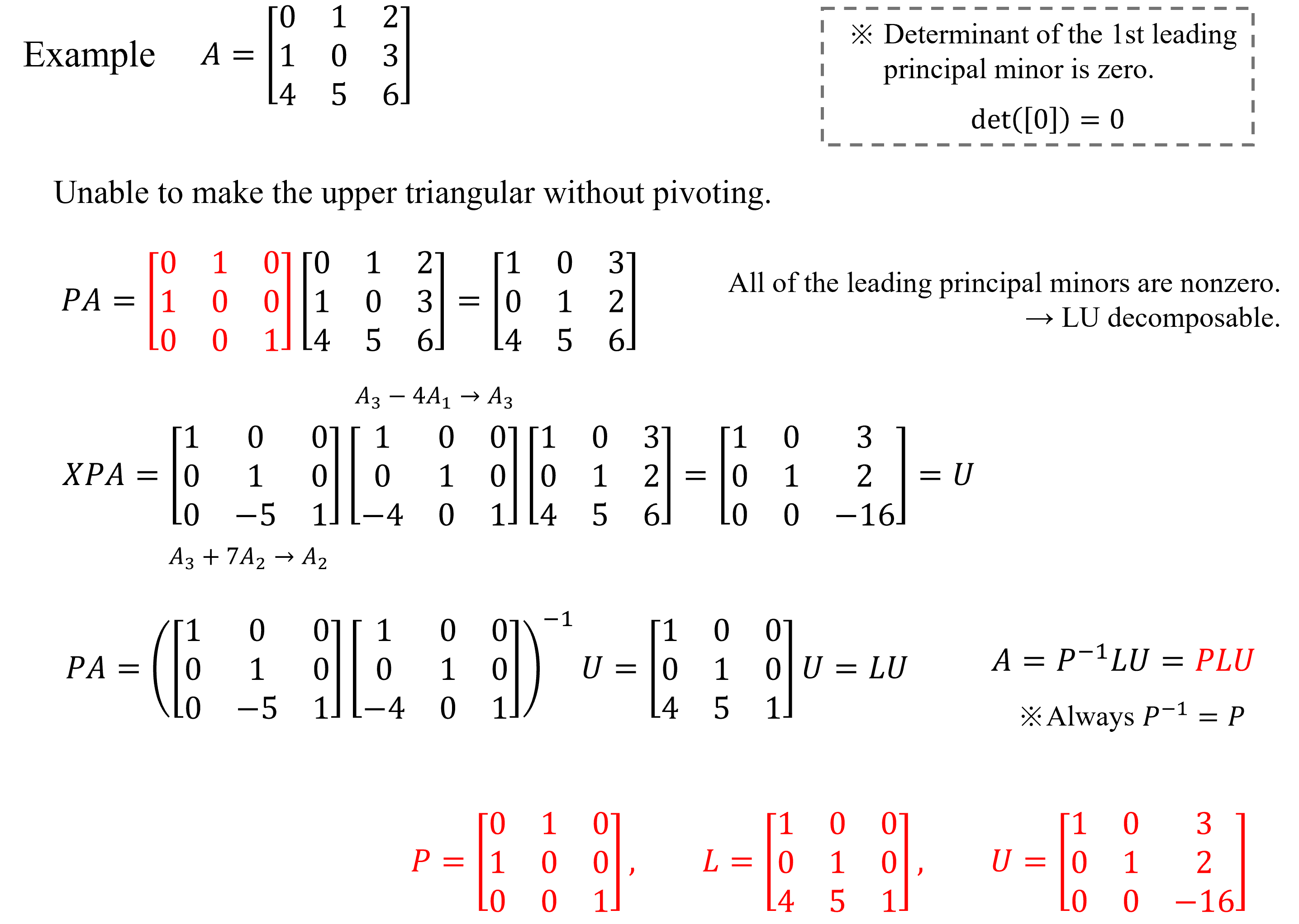
●위처럼 pivoting ($P)$을 섞은 LU decomposition을 PLU decomposition이라 하며, 모든 Square matrix는 PLU decomposition이 가능하다. 마찬가지로 $P$, $L$, $U$는 unique 하지 않다.

 

 

●Uniqueness를 확보하기 위해 LU decomposition 알고리즘들은 $L$의 diagonal elements = 0 등의 조건을 추가하기도 한다. Matlab의 경우 Dolittle's method라는 알고리즘을 사용하여 $L$, $U$를 구한다.

 

 

●Square matrix A가 Symmetric이고 positive definite 하면 $U=L^T$, 즉 $A=LU=LL^{T}$로 분해할 수 있으며 이를 Cholesky decomposition(숄레스키 분해)라고 한다.

 

 

●①Solving systems of linear equations easily, ②Calculate the inverse and determinant easily 등에 사용할 수 있다.

 

 

 

①Solving systems of linear equations easily

●$Ax=b$에서 $A$를 LU decomposition 하면 $LUx=b$로 식을 정리할 수 있다. $Ux=y$로 두면 $Ly=b$식을 얻을 수 있는데, $L$은 lower-triangular matrix이므로 $L^{-1}$를 사용하지 않고 Forward substitution으로 $y$를 쉽게 계산할 수 있다.

 

$\begin{bmatrix}l_{11} & 0 & 0 \\l_{21} & l_{22} & 0 \\l_{31} & l_{32} & l_{33}\end{bmatrix}\begin{bmatrix}y_{1} \\y_{2} \\y_{3}\end{bmatrix}=\begin{bmatrix}b_{1} \\b_{2} \\b_{3}\end{bmatrix}$

 

$y_{1}=b_{1}/l_{11}$,        $y_{2}=(b_{2}-l_{21}y_{1})/l_{22}$,         $y_{3}=(b_{3}-l_{31}y_{1}-l_{32}y_2)/l_{33}$

 

 

●이후 $Ux=y$도 마찬가지로 $U^{-1}$ 사용하지 않고 Backward substitution 최종 해인 $x$를 쉽게 계산할 수 있다.

 

$\begin{bmatrix}u_{11} & u_{12} & u_{13} \\0 & u_{22} & u_{23} \\0 & 0 & u_{33}\end{bmatrix}\begin{bmatrix}x_{1} \\x_{2} \\x_{3}\end{bmatrix}=\begin{bmatrix}y_{1} \\y_{2} \\y_{3}\end{bmatrix}$

 

$x_{3}=y_{3}/u_{33}$,        $x_2=(y_2-u_{23}x_3)/u_{22}$,         $x_1=(y_1-u_{12}x_2-u_{13}x_3)/u_{11}$

 

 

 

②Calculate the inverse and determinant easily

●Triangular matrix는 비교적 역행렬을 구하기 쉽기에 Square matrix A의 역행렬을 구할 때 LU decomposition을 활용하는 알고리즘이 많다.

 

●Triangular matrix의 행렬식은 diagonal element의 곱만으로도 구할 수 있다. 또한 행렬식은 $\text{det}(A)\text{det}(B)=\text{det}(AB)$의 성질을 갖고 있기에 LU decomposition을 이용하면 어떤 행렬의 행렬식을 쉽게 구할 수 있다.

 

 

$\text{det}(A)=\text{det}(L)\text{det}(U)=\text{det}\begin{bmatrix}l_{11} &  & 0 \\\vdots  & \ddots &  \\l_{n1} & \cdots  & l_{nn}\end{bmatrix}*\text{det}\begin{bmatrix}u_{11} & \cdots  & u_{1n} \\& \ddots  & \vdots\\0 && u_{nn}\end{bmatrix}=\prod\limits_{i=1}^{n}l_{ii}\prod\limits_{i=1}^{n}u_{ii}$

 

 

 

 

 

 

 

 

+)Gram-Schmidt process (그람-슈미트 과정)

●QR decomposition을 공부하다 이 개념은 흥미로워서 이해한 것을 정리해 봤다. 물론 사실상 Gram-Schmidt process를 한다는 것이 QR decompostion 한다는 것이다.

 

※Gram-Schmidt process가 QR decomposition을 구하는 유일한 방법은 아니다.

 

 

●Gram-Schmidt process를 한 줄로 정리하면 "Linearly independent vectors(Full-ranked matrix)를 orthonormal vectors(Orthogonal matrix)"로 변환하는 과정이다. 그 아래에 내가 이해한 흐름을 정리했다.

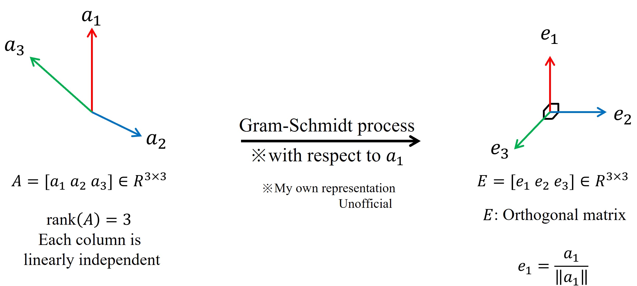
※위 그림과 아래 설명은 $A$가 full-rank인 경우를 예시로 들었다.  반드시 full rank일 필요는 없다. 

 

 

① 기준이 될 벡터$(a_{1})$를 하나 정하고 이를 $u_1$이라 한다. $a_1=u_1$

 

 

② 어떤 벡터가 서로 linearly independent 하지만 orthogonal 하지 않다는 건 한 벡터의 성분을 다른 벡터로 일부 표현할 수 있다는 뜻이다. 기하학적으로는 정사영이 가능하다는 뜻이다.

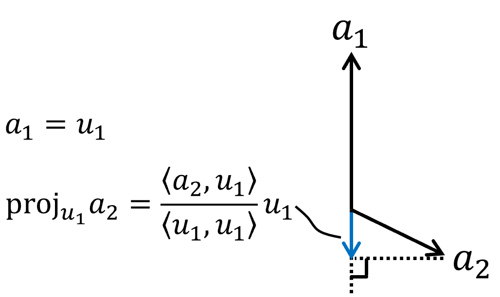
$a_{2}$의 일부는 $a_{1}, a_{3}$으로 표현이 가능한 상황이다.

 

※ <  > 괄호는 내적을 의미한다.

 

 

③ $a_2$에서 $a_1(=u_1)$의 성분을 빼서 만든 벡터($u_2$)를 만들면 더 이상 그 일부를 $a_1(=u_1)$으로는 표현이 불가능, 즉 orthogonal 해진다.

 

$u_2=a_2-\text{proj}_{u_{1}}a_{2}$

 

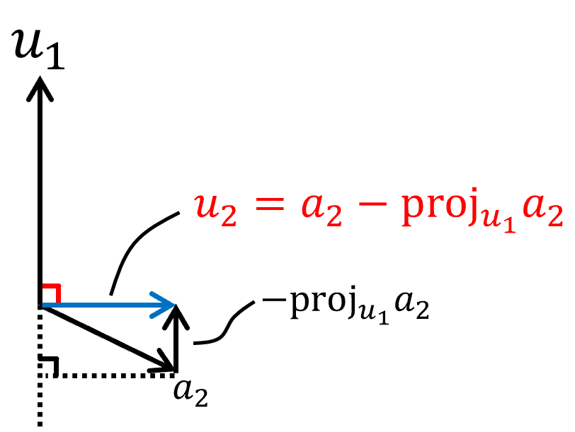
이렇게 $a_1$과 $a_2$의 연결고리(?)를 끊었다. 이제 $u_1$과 $u_2$는 orthogonal 하다.

 

 

④ 한편 $u_2=a_2-\text{proj}_{u_{1}}a_{2}$를 변형하면 $a_2=\text{proj}_{u_{1}}a_{2}+u_2=\frac{\left\langle a_2,u_1 \right\rangle}{\left\langle u_1,u_1 \right\rangle}u_1+u_2$를 알 수 있다.

 

이는 $\color{Red}a_2$는 $\color{Red}u_1$과 $\color{Red}u_2$의 linear combination으로 완전히 표현 가능함을 의미한다.

 

 

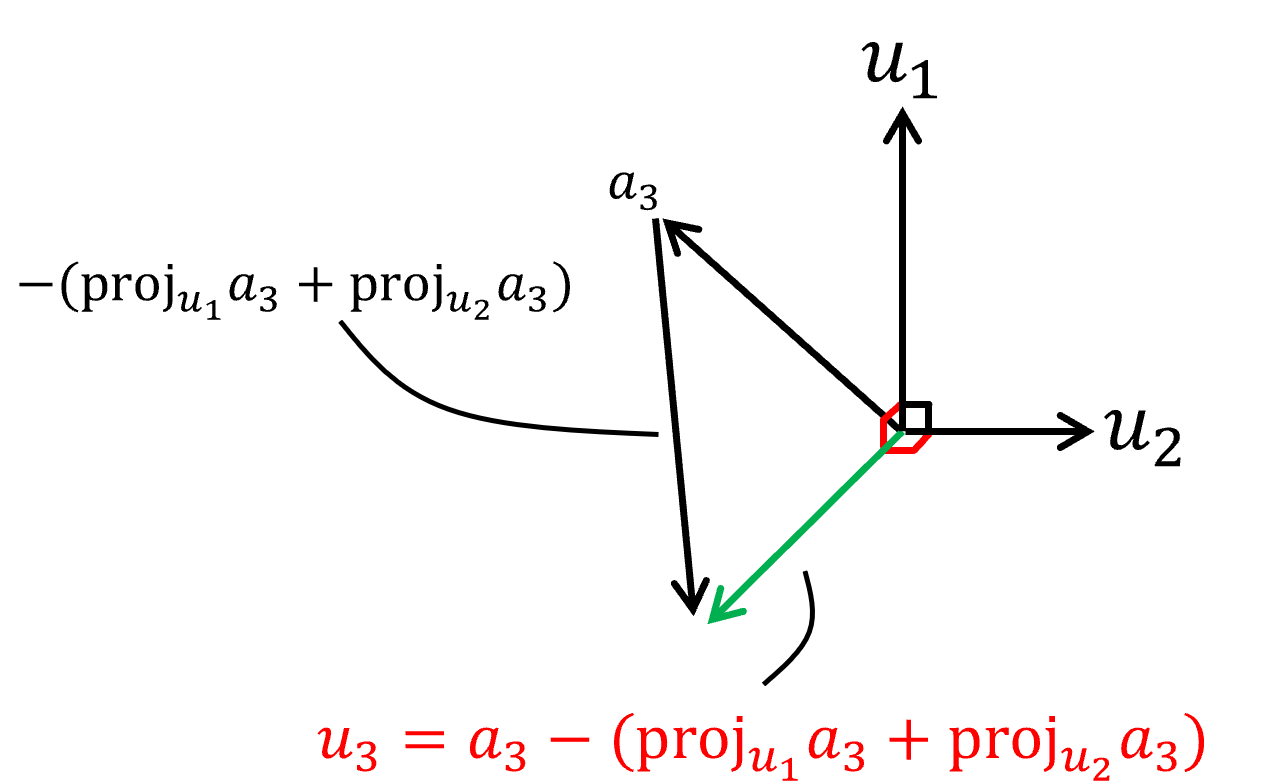
⑤ 이제 남은 $a_3$에는 아직 $a_1=u_1$의 성분과 $a_2$로 부터 만들어진 $u_2$의 성분이 있다.

 

$a_3$도 $u_1$, $u_2$와 orthogonal 하게 만들기 위해 $u_1$, $u_2$의 성분을 빼준다.

 

$u_3=a_1-\text{proj}_{u_{1}}a_{3}-\text{proj}_{u_{2}}a_{3}$

 

 

마찬가지로 $u_3=a_1-\text{proj}_{u_{1}}a_{3}-\text{proj}_{u_{2}}a_{3}$를 변형하여 얻은 식에서  $\color{Red}a_3$는 $\color{Red}u_1$,  $\color{Red}u_2$, $\color{Red}u_3$의 linear combination으로 완전히 표현 가능함을 알 수 있다.

 

 

⑥ $U=\begin{bmatrix}u_1 & u_2 & u_3\end{bmatrix}$의 각 column은 orthogonal 하지만 그 크기가 1이 아니므로 각각 normalize를 해줘서 $e=\begin{bmatrix}e_1 & e_2 & e_3\end{bmatrix}$를 구한다.

 

 

 

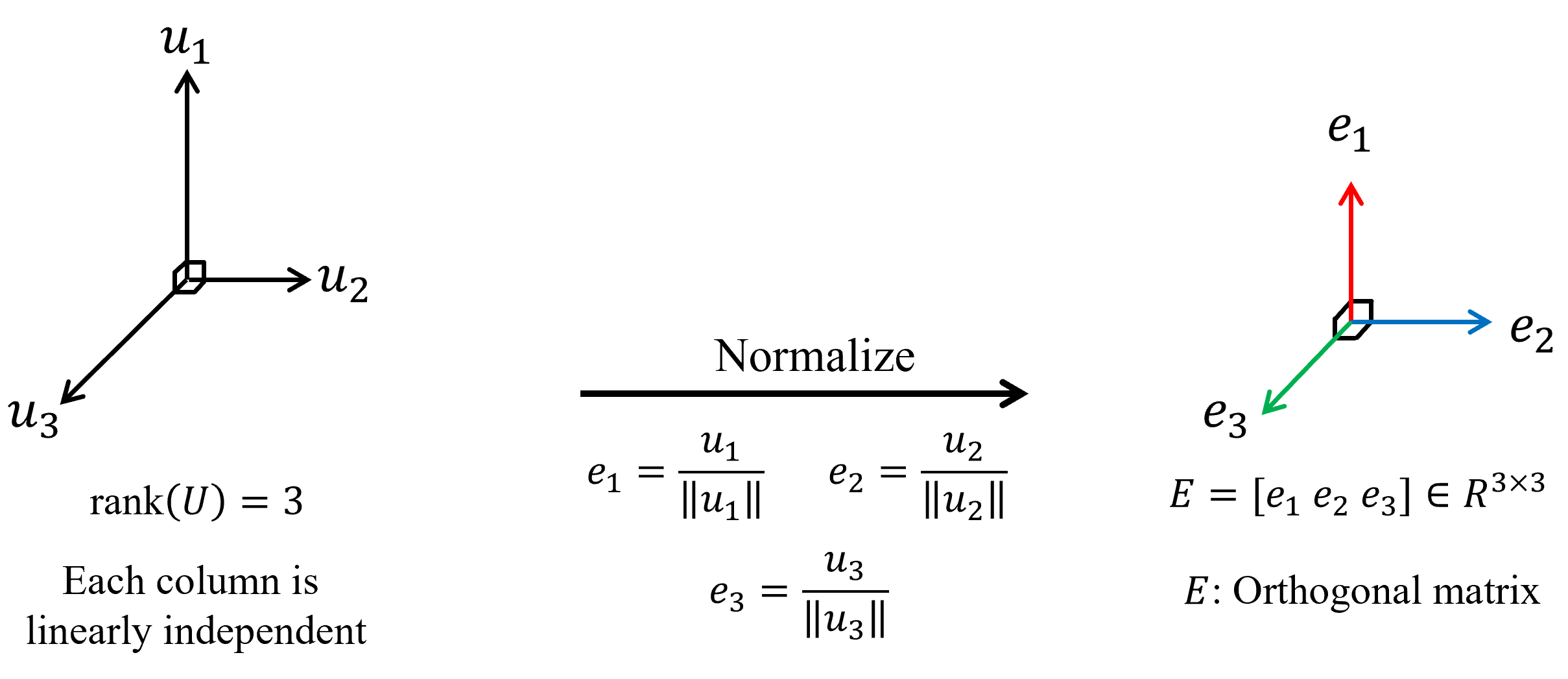
⑦ ①-⑥과정을 통해 얻은 정보는 "$\color{Red}a_1$, $\color{Red}a_2$, $\color{Red}a_3$는 orthonormal vectors $\color{Red}e_1$, $\color{Red}e_2$, $\color{Red}e_3$의 linear combination으로 표현할 수 있다."와 "$\color{Red}a_i$는 $\color{Red}e_1$부터 $\color{Red}e_i$까지의 i개 벡터 성분만을 갖고 있다."이다.

 

다시 간단하게 정사영을 생각해 보면, $a_i$의 $e_1$성분은 내적을 이용하여 $\left\langle a_i,e_1 \right\rangle$로 나타낼 수 있고 '벡터=크기×단위벡터'에 따라 $\left\langle a_i,e_1 \right\rangle e_1$로 쓸 수 있다.

 

즉 $a_i$벡터를 $a_i=\left\langle a_i,e_1 \right\rangle e_1+\left\langle a_i,e_2 \right\rangle e_2+\cdots +\left\langle a_i,e_i \right\rangle e_i=\sum\limits_{r=1}^{i}\left\langle  a_i,e_r\right\rangle e_r$로 완전히 나타낼 수 있다.

 

 

⑧ 다시 위에서 예로 들었던 3차원 벡터를 예로 설명해 보면, 

 

$a_1=\left\langle a_1,e_1 \right\rangle e_1$

$a_2=\left\langle a_2,e_1 \right\rangle e_1+\left\langle a_2,e_2 \right\rangle e_2$

$a_3=\left\langle a_3,e_1 \right\rangle e_1+\left\langle a_3,e_2 \right\rangle e_2+\left\langle a_3,e_3 \right\rangle e_3$

 

$A=\begin{bmatrix} a_1 & a_2 & a_3 \end{bmatrix}=\begin{bmatrix} e_1 & e_2 & e_3 \\ \end{bmatrix}\begin{bmatrix} \left\langle a_1,e_1 \right\rangle & \left\langle a_2,e_1 \right\rangle & \left\langle a_3,e_1 \right\rangle \\  0 & \left\langle a_2,e_2 \right\rangle  & \left\langle a_3,e_2 \right\rangle \\ 0 & 0 & \left\langle a_3,e_3 \right\rangle \end{bmatrix}=EU$

 

※$U\text{: Upper-triangular matrix}$

 

 

 

 

QR decomposition(QR decomposition, QR 분해)

모든 matrix A($m\times n$)는 다음과 같이 분해할 수 있다.

 

$A=QR$       $Q\text{: Orthogonal matrix}$,    $R\text{: Upper-triangular matrix}$

 

※$Q$는 $A$에 Gram-Schmidt process를 적용해 얻은 $E$이고, $R$은 $U$이다. 왜 굳이 QR로 했는지는 모르겠다..

 

 

●$A$가 Square matrix $(n\times n)$인 경우 $Q, R\in \mathbb{R}^{n\times n}$로 분해할 수 있다. $Q$와 $R$의 각 column의 의미는 위 Gram-Schmidt process의 ⑦에 자세히 설명해 뒀다.

 

 

●QR decomposition을 구하는 방법은 크게 Gram-Schmidt process와 Householder method가 있다. 일반적으로는 Householder method를 이용한 알고리즘을 사용하는데 이는 Gram-Schmidt보다 numerically stable 한 방식이기 때문이다. Matlab의 qr 명령어도 Householder method를 사용한다고 한다.

 

 

●$A$가 Rectangular matrix $(\color{Red} m\times n, m \gt n)$인 경우에는 2가지 QR decomposition을 구할 수 있다. 

 

 

 

ⓐ Reduced QR decomposition

●$Q \in \mathbb{R}^{m\times n}$,    $R\in \mathbb{R}^{n\times n}$

 

●이 경우는 Gram-Schmidt process을 그대로 따랐을 때 구할 수 있는 QR decomposition이다. 반대로 말하면 Gram-Schmidt만으로는 오직 Reduced QR decomposition밖에 구할 수 없다.

 

●n개의 m차원 벡터를 가진 $A$로부터 n개의 orthonormal m차원 벡터를 가진 $Q$를 만들어 낸다. (=차원을 유지한다.)

 

●예를 들어 2개의 3차원 벡터로 이루어진 $A \in \mathbb{R}^{3\times 2}$는 3차원 공간에 2차원 평면을 만든다. 이 $A$에서 얻은 $Q$또한 $Q \in \mathbb{R}^{3\times 2}$로 3차원 공간에 단위벡터가 orthogonal 한 2차원 평면을 만든다. (Not good enough)

 

$A=\begin{bmatrix} 2 & 4 \\ 3 & 1 \\ 6 & 5 \end{bmatrix}=\begin{bmatrix} 0.29 & 0.84 \\ 0.43 & -0.54 \\ 0.86 & -0.01 \end{bmatrix}\begin{bmatrix} 7 & 5.86 \\ 0 & 2.77 \end{bmatrix}=QR$

 

 

 

 

ⓑ Full QR decomposition

●$Q \in \mathbb{R}^{ \color{Red}  m\times m} , R\in \mathbb{R}^{ \color{Red}  m\times n}$이고 $R$의 마지막 $m-n$row는 모두 0이다

 

●n개의 m차원 벡터를 가진 $A$로부터 m개의 orthonormal 차원 벡터를 가진 $Q$를 만들어 낸다. (=차원을 m-n만큼 증가시킨다.)

 

●한편 새로 얻은 차원($Q$의 마지막 column)은 dummy로 원래의 $A$의 벡터(column)들을 표현하는 데에 전혀 필요 없다. 그래도 이 새로운 column 역시 다른 column과 orthonormal 하므로 full QR decomposition의 Q 역시 orthogonal matrix이다.

 

●2개의 3차원 벡터로 이루어진 $A \in \mathbb{R}^{3\times 2}$는 3차원 공간에 2차원 평면을 만든다. 이 $A$에서 full QR decomposition으로 얻은 $Q\in\mathbb{R}^{3\times 3}$는 단위벡터가 orthogonal 한 3차원 공간을 만든다. 하지만 그 공간의 한 방향(dummy column)은 원래의 3차원 공간상의 2차원 평면 $A$를 표현하는 데에 전혀 필요 없다.

 

●Gram-Schmidt로 Reduced QR decomposition을 구한 경우 $Q$의 column과 orthonormal 한 벡터를 하나 만들어 Q에 추가해 주고, $R$의 아래쪽에는 0을 추가해 Full QR decomposition을 구할 수 있다.

 

$A=\begin{bmatrix} 2 & 4 \\ 3 & 1 \\ 6 & 5 \end{bmatrix}=\begin{bmatrix} 0.29 & 0.84 \\ 0.43 & -0.54 \\ 0.86 & -0.01 \end{bmatrix}\begin{bmatrix} 7 & 5.86 \\ 0 & 2.77 \end{bmatrix}$

 

$q_{dummy}=q_1\times q_2=\begin{bmatrix} 0.46 \\ 0.73 \\ -0.52 \end{bmatrix}$   (※간단하게 cross product으로 구했다.)

 

$Q'=\begin{bmatrix} 0.29 & 0.84 & 0.46\\ 0.43 & -0.54 & 0.73\\ 0.86 & -0.01 & -0.52\end{bmatrix}$

 

$\begin{bmatrix} R \\ 0 \end{bmatrix}=\begin{bmatrix} 7 & 5.86 \\ 0 & 2.77 \\ 0 & 0 \end{bmatrix}$

 

$A=Q'\begin{bmatrix} R \\ 0 \end{bmatrix}$

 

●아래 유튜브 영상에서 Reduced QR과 Full QR의 차이를 예시를 들어 쉽게 설명해뒀다.

 

https://www.youtube.com/watch?v=RkoFIxk_LXI

 

 

 

 

 

 

 

 

 

●①Solving systems of linear equations easily, ②Solving least square problems 등에 사용할 수 있다.

 

① Solving systems of linear equations easily

 

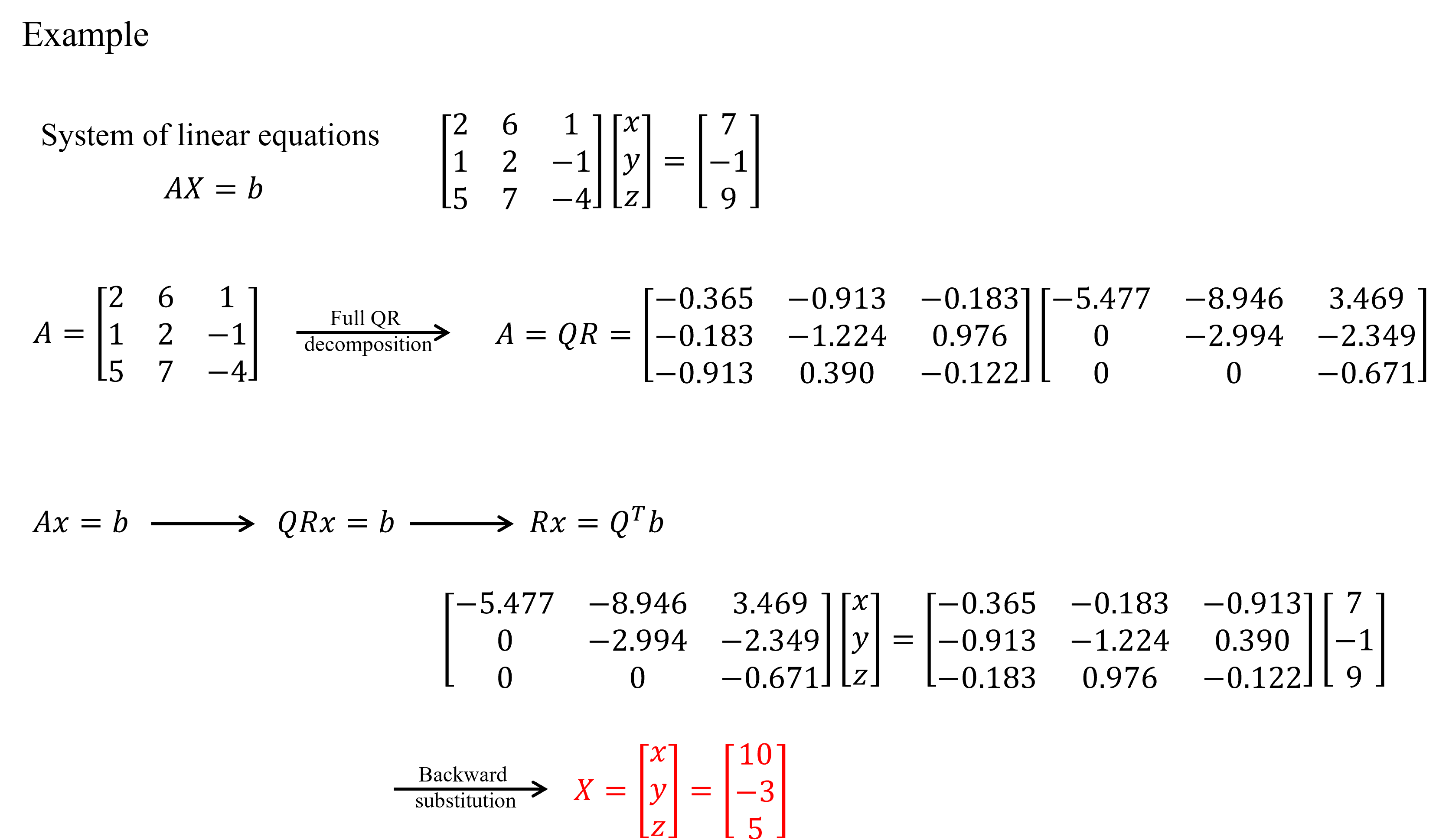
●$Ax=b$ $(A \in \mathbb{R}^n\times n)$에서 $A$를 QR decomposition 하면 $QRx=b$로 식을 정리할 수 있다. $Q$는 orthogonal matrix이기에 $Q^{-1}=Q^T$을 이용할 수 있고, $R$은 upper triangular matrix이기에 backward substituition을 이용할 수 있다.

 

 

 

 

 

 

 

 

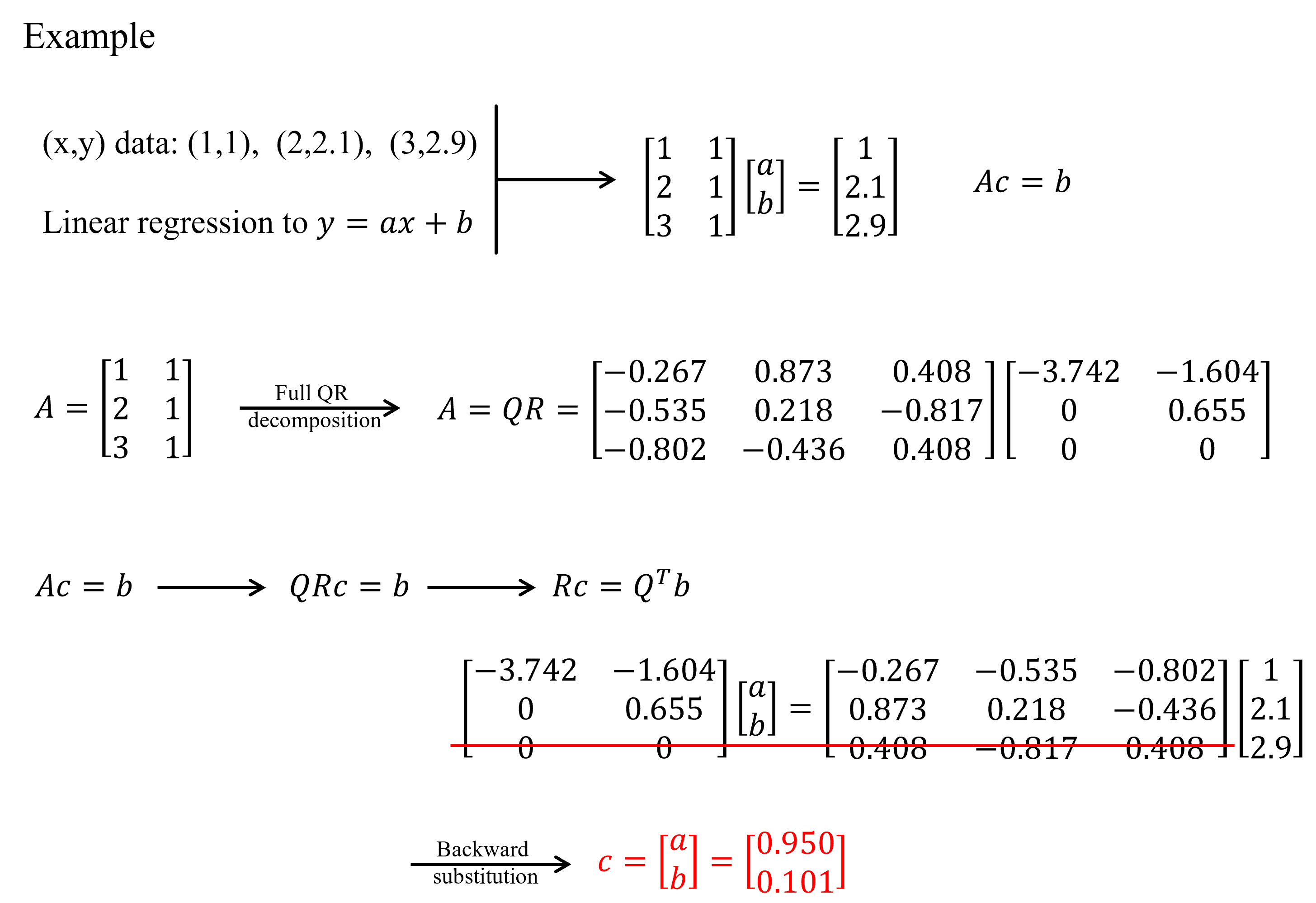
② Solving least square problems

 

※ Systems of linear equations problem과 Least square problem은 둘 다 $Ax=b$ equation을 다루는 문제인데 그 차이를 한 줄로 설명하면 아래와 같다. (불확실)

 

"In the matrix equation $Ax=b$ ($A \in \mathbb{R}^{m \times n}$), when $m=n$, it's a system of linear equations. When $m>n$, it becomes an overdetermined system best solved using the least square method to find an approximate solution."

 

 

●$Ax=b$ $(A \in \mathbb{R}^m\times n)$  $(m \le n)$에서 $A$를 Full QR decomposition하여 Q와 R을 얻은 후 ①과 같은 과정을 거치면 approximate solution을 구할 수 있다. 이때 dummy로 생긴 row는 빼고 계산한다.

 

 

●당연히 linear regression에도 이용할 수 있다.

 

 

 

 

 

 

 

 

 

 

 

 

 

 

 

https://en.wikipedia.org/wiki/LU_decomposition#Example

LU decomposition - Wikipedia

(25.01.16 접속)

 

 

https://www.cfm.brown.edu/people/dobrush/cs52/Mathematica/Part2/PLU.html

https://www.cfm.brown.edu/people/dobrush/cs52/Mathematica/Part2/PLU.html

(25.01.16 접속)

 

 

https://angeloyeo.github.io/2021/06/16/LU_decomposition.html

LU 분해 - 공돌이의 수학정리노트 (Angelo's Math Notes)

(25.01.16 접속)

 

 

https://en.wikipedia.org/wiki/QR_decomposition

QR decomposition - Wikipedia

(25.01.16 접속)

 

 

https://angeloyeo.github.io/2020/11/23/gram_schmidt.html

QR 분해 - 공돌이의 수학정리노트 (Angelo's Math Notes)

(25.01.16 접속)

 

 

https://www.youtube.com/watch?v=RkoFIxk_LXI

 

(25.01.16 접속)

 

 

Dennis G. Zill, "Advanced Engineering Mathematics" 6th international student edition, 2017. 

 

 

 

========================================================================
정확한 정보 전달보단 공부 겸 기록에 초점을 둔 글입니다.
틀린 내용이 있을 수 있습니다.
틀린 내용이나 다른 문제가 있으면 댓글에 남겨주시면 감사하겠습니다. : )
========================================================================